import numpy as np
import matplotlib.pyplot as plt
from stable_baselines3 import SAC
from stable_baselines3.common.monitor import Monitor
from stable_baselines3.common.callbacks import BaseCallback
from common import (
    ornstein_uhlenbeck,
    TradingEnv,
    buy_and_hold,
    evaluate_policy_on_env,
    sharpe_ratio,
    max_drawdown,
    plot_learning_curve,
    plot_equity_curves,
    plot_price_and_positions,
)
SEED = 0
TRAIN_SEED = 1
TEST_SEED = 999
N_TRAIN = 5000
N_TEST = 3000
WINDOW = 20
COST = 0.0005
TOTAL_STEPS = 60_000Lesson 7 — Continuous position SIZING with SAC
Every agent so far chose a direction: short, flat, or long — three discrete buttons. But a real desk does not just decide which way; it decides how much. Half a unit of conviction should buy half a position. Sizing is risk control, and it is where FX trading actually lives. So we replace the three buttons with a continuous dial: a target position anywhere in [-1, +1].
That one change breaks DQN. DQN works by taking argmax over actions — trivial when there are three, impossible when there are infinitely many points in an interval. Continuous control needs a different algorithm class: an actor-critic that outputs an action directly instead of scoring a finite menu.
Enter SAC: Soft Actor-Critic
SAC (Soft Actor-Critic) is an off-policy actor-critic for continuous control. It keeps two moving parts:
- an actor (the policy) that maps a state to a distribution over actions and samples the position to take, and
- a critic (a Q-network, in fact two of them, to fight over-optimism) that scores how good a (state, action) pair is.
Its defining trick is maximum-entropy RL: SAC maximises reward plus the policy’s entropy. In plain terms it is rewarded for staying as random as it can get away with while still succeeding. That built-in pressure to stay stochastic makes it explore thoroughly, learn from a replay buffer sample- efficiently, and end up robust rather than brittle. An automatically tuned “temperature” trades entropy off against reward as training proceeds.
The deterministic cousins
DDPG and TD3 solve the same continuous-control problem with a deterministic actor (one action, no distribution) plus hand-added exploration noise. TD3 is essentially DDPG made stable (twin critics, delayed updates). SAC’s entropy bonus usually makes it the more forgiving default — and it is the algorithm class we reach for in the FX capstone.
We train on one mean-reverting Ornstein-Uhlenbeck path and, as always, judge the agent only on a held-out path it has never seen.
Run order matters. The cells below build on each other. Run them top to bottom (Jupyter: Run → Run All Cells; VS Code: Run All). If you hit
NameError(or similar), you skipped the Setup cell — run it first.
Setup — imports & configuration
Run this cell first. It imports every library and defines the module-level constants the rest of the notebook relies on.
RewardLoggerCallback (class)
Collect per-episode rewards from the Monitor wrapper during training.
Stable-Baselines3’s Monitor writes a summary dict into info["episode"] the moment an episode ends ("r" = total reward, "l" = length). This callback fires on every environment step, watches the infos that SB3 exposes in self.locals, and stashes each finished episode’s reward. That growing list is our learning curve — the honest record of whether training is improving the policy or just burning GPU cycles.
class RewardLoggerCallback(BaseCallback):

    def __init__(self):
        super().__init__()
        self.episode_rewards = []

    def _on_step(self):
        for info in self.locals.get("infos", []):
            episode = info.get("episode")
            if episode is not None:
                self.episode_rewards.append(episode["r"])
        return True
make_prices (function)
One mean-reverting Ornstein-Uhlenbeck price path from a given seed.
The seed is the whole point: calling this with two different seeds gives two statistically similar but independent markets. We train on one and test on the other — the only honest way to ask “did the agent learn a rule, or memorise a path?”.
def make_prices(n, seed):
    rng = np.random.default_rng(seed)
    return ornstein_uhlenbeck(n, rng, mu=1.0, theta=0.05, sigma=0.01)
train_sac (function)
Train a SAC agent on the continuous-action training environment.
These are standard SAC settings for a small MLP on a dense reward:
learning_rate=3e-4— the usual Adam step for both actor and critics.buffer_size=100_000withlearning_starts=1000— SAC is off-policy, so it replays a large pool of past transitions; fill it a little before training so early gradients are not dominated by one trajectory.batch_size=256— big minibatches keep the critic updates low-variance.gamma=0.99— value future PnL almost as much as present PnL.tau=0.005— Polyak coefficient; the target critics track the live critics slowly, which is what keeps bootstrapped values from diverging.train_freq=1,gradient_steps=1— one gradient update per env step, the setting that makes SAC so sample-efficient.
The entropy temperature is auto-tuned by default, so we do not set it: SAC decides for itself how stochastic to stay. Returns the trained model and the list of per-episode training rewards.
def train_sac(train_env, total_steps, seed):
    logger = RewardLoggerCallback()
    model = SAC(
        "MlpPolicy",
        train_env,
        learning_rate=3e-4,
        buffer_size=100_000,
        learning_starts=1000,
        batch_size=256,
        gamma=0.99,
        tau=0.005,
        train_freq=1,
        gradient_steps=1,
        device="auto",
        seed=seed,
        verbose=0,
    )
    model.learn(total_timesteps=total_steps, callback=logger, progress_bar=False)
    return model, logger.episode_rewards
report_metrics (function)
Print the three numbers a trader actually judges a strategy by.
def report_metrics(label, metrics):
    print(
        f"{label:14s} | total PnL = {metrics['total_pnl']:+.4f} "
        f"| Sharpe = {metrics['sharpe']:+.2f} "
        f"| max drawdown = {metrics['max_drawdown']:+.4f}"
    )
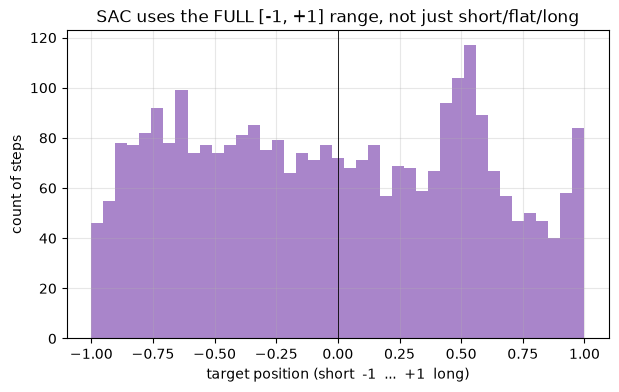
plot_position_histogram (function)
Histogram of the continuous positions the agent chose.
This is the figure that proves the point of the whole lesson. A discrete agent can only ever land on -1, 0, or +1, so its histogram would be three spikes. A continuous agent that has genuinely learned to size spreads its mass across the whole [-1, +1] dial — scaling how much it holds with how confident it is, not just picking a direction.
def plot_position_histogram(positions, title="Agent position sizes (held-out)", ax=None):
    if ax is None:
        _, ax = plt.subplots(figsize=(7, 4))
    ax.hist(positions, bins=41, range=(-1.0, 1.0), color="tab:purple", alpha=0.8)
    ax.axvline(0, color="k", lw=0.6)
    ax.set_xlabel("target position (short  -1  ...  +1  long)")
    ax.set_ylabel("count of steps")
    ax.set_title(title)
    ax.grid(alpha=0.3)
    return ax
main (function)
def main():
    np.random.seed(SEED)

    # --- Build TRAIN and HELD-OUT TEST markets from DIFFERENT seeds ---------
    train_prices = make_prices(N_TRAIN, TRAIN_SEED)
    test_prices = make_prices(N_TEST, TEST_SEED)
    print(
        f"Train path: {N_TRAIN} bars (seed {TRAIN_SEED}) | "
        f"Held-out test path: {N_TEST} bars (seed {TEST_SEED})"
    )

    # Continuous action space + a risk-adjusted (Sharpe) reward. Monitor wraps
    # the training env so finished-episode rewards are logged for the curve.
    train_env = Monitor(
        TradingEnv(train_prices, window=WINDOW, cost=COST,
                   continuous=True, reward="sharpe")
    )

    # --- Train ------------------------------------------------------------
    print(f"\nTraining SAC for {TOTAL_STEPS:,} steps (device=auto)...")
    model, episode_rewards = train_sac(train_env, TOTAL_STEPS, SEED)
    print(f"Done. Logged {len(episode_rewards)} training episodes.")

    # --- Evaluate on the HELD-OUT test path -------------------------------
    # Fresh continuous env on the test prices: never-before-seen returns.
    test_env = TradingEnv(test_prices, window=WINDOW, cost=COST,
                          continuous=True, reward="sharpe")
    agent = evaluate_policy_on_env(model, test_env, deterministic=True)

    # Buy-and-hold (always +1) on the SAME held-out env is the baseline to beat.
    bh_env = TradingEnv(test_prices, window=WINDOW, cost=COST,
                        continuous=True, reward="sharpe")
    bh_pnls = buy_and_hold(bh_env)
    bh_metrics = {
        "total_pnl": float(np.sum(bh_pnls)),
        "sharpe": sharpe_ratio(bh_pnls),
        "max_drawdown": max_drawdown(bh_pnls),
    }

    print("\nHeld-out test performance:")
    report_metrics("SAC agent", agent)
    report_metrics("buy & hold", bh_metrics)

    positions = np.asarray(agent["positions"], dtype=np.float64)
    print(
        f"\nAgent position range: [{positions.min():+.2f}, {positions.max():+.2f}]"
        f"  |  mean |position| = {np.abs(positions).mean():.2f}  "
        f"(a discrete agent could only ever print -1, 0, or +1)"
    )

    # --- Figure 1: learning curve -----------------------------------------
    plot_learning_curve(
        episode_rewards, window=10,
        title="SAC training — episode reward over time",
    )
    plt.show()

    # --- Figure 2: equity curves on held-out data -------------------------
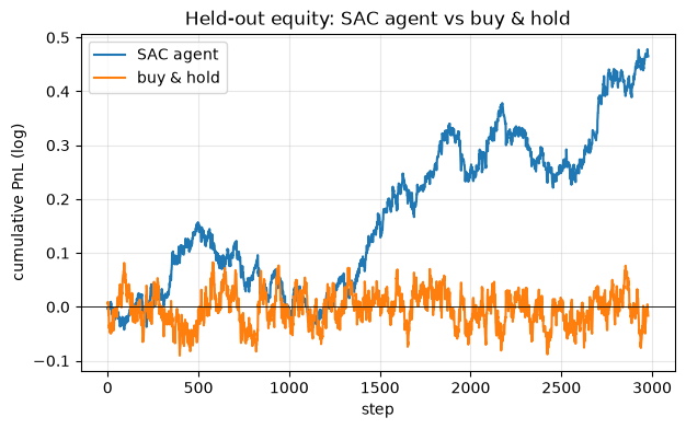
    plot_equity_curves(
        {"SAC agent": agent["pnls"], "buy & hold": bh_pnls},
        title="Held-out equity: SAC agent vs buy & hold",
    )
    plt.show()

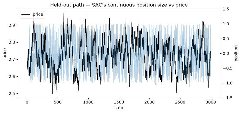
    # --- Figure 3: the CONTINUOUS position varying smoothly with price ----
    plot_price_and_positions(
        test_prices, agent["positions"],
        title="Held-out path — SAC's continuous position size vs price",
    )
    plt.show()

    # --- Figure 4: the histogram that proves it uses the whole dial -------
    plot_position_histogram(
        agent["positions"],
        title="SAC uses the FULL [-1, +1] range, not just short/flat/long",
    )
    plt.show()

    # --- Takeaway ---------------------------------------------------------
    print(
        "\nTakeaway: making the action a continuous target position turns "
        "direction-picking into position SIZING — the agent scales how much it "
        "holds with its conviction, which is the essence of risk control. DQN "
        "cannot do this (there is no argmax over a continuous interval), so we "
        "switched to SAC: an off-policy actor-critic that maximises reward PLUS "
        "policy entropy, exploring by staying as stochastic as it can while still "
        "succeeding. That makes it sample-efficient and robust. DDPG/TD3 are its "
        "deterministic cousins. Watch the position histogram: the mass spread "
        "across [-1, +1] is the whole point — and SAC is the algorithm class we "
        "carry into the FX capstone."
    )
Run the lesson
Execute everything above, then run main().
main()Train path: 5000 bars (seed 1) | Held-out test path: 3000 bars (seed 999)
Training SAC for 60,000 steps (device=auto)...
Done. Logged 12 training episodes.
Held-out test performance:
SAC agent | total PnL = +0.4650 | Sharpe = +0.45 | max drawdown = -0.1892
buy & hold | total PnL = -0.0165 | Sharpe = -0.01 | max drawdown = -0.1720
Agent position range: [-1.00, +1.00] | mean |position| = 0.49 (a discrete agent could only ever print -1, 0, or +1)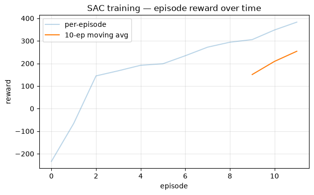
Takeaway: making the action a continuous target position turns direction-picking into position SIZING — the agent scales how much it holds with its conviction, which is the essence of risk control. DQN cannot do this (there is no argmax over a continuous interval), so we switched to SAC: an off-policy actor-critic that maximises reward PLUS policy entropy, exploring by staying as stochastic as it can while still succeeding. That makes it sample-efficient and robust. DDPG/TD3 are its deterministic cousins. Watch the position histogram: the mass spread across [-1, +1] is the whole point — and SAC is the algorithm class we carry into the FX capstone.