import gymnasium as gym
import numpy as np
import torch
import torch.nn as nn
import matplotlib.pyplot as plt
from stable_baselines3 import A2C
from stable_baselines3.common.monitor import Monitor
from stable_baselines3.common.callbacks import BaseCallback
from stable_baselines3.common.evaluation import evaluate_policy
from common import plot_learning_curve
SEED = 0
ENV_ID = "CartPole-v1"
DEVICE = "cpu"
REINFORCE_EPISODES = 800
GAMMA = 0.99
LR = 1e-3
HIDDEN = 128
GRAD_CLIP = 0.5
A2C_STEPS = 100_000
EVAL_EPISODES = 20Lesson 5 — Policy gradients: REINFORCE from scratch, then A2C
Every method so far has been value-based. The bandits estimated an action-value Q; DQN (L3/L4) learned a Q-network and acted greedily on it. The policy was always a side-effect: derive the action by taking an argmax over values. This lesson flips that around. We now learn the policy directly — a parameterised function pi(a | s) that outputs action probabilities — and push its parameters straight up the gradient of expected return. No value table, no argmax. This is the policy-gradient family, and it is what modern RL (PPO, the algorithm behind RLHF) is built on.
Why bother, when DQN works? Three reasons that matter later:
- policies can be stochastic by construction — useful when the optimal play is to randomise (bluffing, exploration, partially-observed markets),
- they extend cleanly to continuous actions (no argmax over infinitely many actions), and
- they optimise the thing we actually care about — return — without ever needing accurate value estimates as an intermediate.
We change environments to make the ideas crisp. Instead of the trading env we use Gymnasium’s CartPole-v1: balance a pole on a cart by pushing left or right, +1 reward per timestep upright, episode ends when it falls (max 500 steps). It is the hello-world of policy gradients because “learning” is unmistakable — the pole stays up longer and longer.
The lesson has two halves:
Part 1 — REINFORCE, hand-built in PyTorch
The pedagogical core. We implement the policy-gradient theorem ourselves in ~40 lines: a small network, sample actions, weight each action’s log-probability by the return it led to, and step. You will see exactly why it works and exactly why it is noisy.
Part 2 — A2C, via Stable-Baselines3
The practical, lower-variance cousin. An Actor-Critic learns a value critic alongside the policy and uses it as a baseline, cutting the variance that plagues REINFORCE and letting us update online instead of waiting for whole episodes. We let SB3 do the heavy lifting and simply watch it learn faster and steadier — then contrast the two in the takeaways.
Run order matters. The cells below build on each other. Run them top to bottom (Jupyter: Run → Run All Cells; VS Code: Run All). If you hit
NameError(or similar), you skipped the Setup cell — run it first.
Setup — imports & configuration
Run this cell first. It imports every library and defines the module-level constants the rest of the notebook relies on.
PolicyNetwork (class)
A small MLP that maps a state to action logits — the policy pi.
Two hidden layers of HIDDEN units with tanh non-linearities, then a linear head producing one logit per action. We deliberately output logits, not probabilities: torch.distributions.Categorical will turn them into a proper distribution (via softmax) and, crucially, give us the log_prob(a) term the policy-gradient update needs.
Note what is absent: there is no value head, no Q. The network’s only job is “given this state, how should I hedge my bets over actions?” For CartPole the state is 4 numbers (cart position/velocity, pole angle/velocity) and there are 2 actions (push left, push right).
class PolicyNetwork(nn.Module):

    def __init__(self, obs_dim, n_actions, hidden=HIDDEN):
        super().__init__()
        self.net = nn.Sequential(
            nn.Linear(obs_dim, hidden),
            nn.Tanh(),
            nn.Linear(hidden, hidden),
            nn.Tanh(),
            nn.Linear(hidden, n_actions),
        )

    def forward(self, obs):
        return self.net(obs)
select_action (function)
Sample an action from the policy and return it with its log-probability.
This is the heart of a stochastic policy. We push the state through the network to get logits, wrap them in a Categorical distribution, and sample — we do not take the argmax. Sampling is what gives REINFORCE its exploration for free: early on the distribution is near-uniform, so the agent tries both actions; as training sharpens the logits it commits to good ones.
We return log pi(a | s) because the policy-gradient update needs the gradient of the log-probability of the action we actually took. Keeping the differentiable log_prob tensor (not just the integer action) lets loss.backward() flow gradients back into the network weights.
def select_action(policy, state):
    state_t = torch.as_tensor(state, dtype=torch.float32, device=DEVICE)
    logits = policy(state_t)
    dist = torch.distributions.Categorical(logits=logits)
    action = dist.sample()
    return int(action.item()), dist.log_prob(action)
discounted_returns (function)
Compute the return-to-go G_t for every timestep of an episode.
G_t = r_t + gamma*r_{t+1} + gamma^2*r_{t+2} + ... — the total discounted reward from step t onward. This is the credit each action gets: an action is judged by everything that happened after it, not before (what came before was not its doing). We build it in one backward pass, accumulating from the end of the episode.
Why return-to-go and not the whole-episode return for every step? Because it is a lower-variance, still-unbiased weighting: action a_t only takes responsibility for rewards it could have influenced.
def discounted_returns(rewards, gamma=GAMMA):
    G = 0.0
    out = np.empty(len(rewards), dtype=np.float64)
    for t in reversed(range(len(rewards))):
        G = rewards[t] + gamma * G
        out[t] = G
    return out
run_reinforce (function)
Train a policy with REINFORCE, the Monte-Carlo policy gradient.
The algorithm, in full:
- Run one complete episode with the current policy, recording each step’s
log pi(a_t | s_t)and reward. - Compute the return-to-go
G_tfor every step. - Form the loss
-sum_t log pi(a_t | s_t) * G_tand take one Adam step.
Step 3 is the policy-gradient theorem in code. The gradient of expected return equals E[ sum_t grad log pi(a_t|s_t) * G_t ]. Read it plainly: push up the log-probability of actions that were followed by high return, push down those followed by low return, each scaled by how high or low. Over many episodes the policy drifts toward whatever earns more. We minimise the negative because PyTorch optimisers descend.
The variance problem, and the baseline fix. Raw G_t values are all positive here (every upright step adds +1), so every action gets pushed up — only the relative sizes teach anything, and they are swamped by noise. The cure is a baseline b: subtract it from the returns so the update uses G_t - b. Any baseline that does not depend on the action leaves the gradient unbiased but can slash its variance. Here we use the cheapest useful one: standardise the returns to zero mean and unit variance within the episode. Now good-relative-to-average actions get pushed up and bad ones get pushed down, and the scale is tamed. (Part 2’s A2C replaces this crude baseline with a learned value function — a strictly better estimate of the average return from each state.)
def run_reinforce(episodes=REINFORCE_EPISODES, seed=SEED):
    torch.manual_seed(seed)
    np.random.seed(seed)

    env = gym.make(ENV_ID)
    obs_dim = env.observation_space.shape[0]
    n_actions = env.action_space.n

    policy = PolicyNetwork(obs_dim, n_actions).to(DEVICE)
    optimizer = torch.optim.Adam(policy.parameters(), lr=LR)

    episode_returns = []
    for ep in range(episodes):
        state, _ = env.reset(seed=seed + ep)
        log_probs, rewards = [], []
        done = False
        while not done:
            action, log_prob = select_action(policy, state)
            state, reward, terminated, truncated, _ = env.step(action)
            done = terminated or truncated
            log_probs.append(log_prob)
            rewards.append(reward)

        episode_returns.append(sum(rewards))

        # Return-to-go, then standardise as a variance-reducing baseline.
        G = discounted_returns(rewards, GAMMA)
        G = torch.as_tensor(G, dtype=torch.float32, device=DEVICE)
        G = (G - G.mean()) / (G.std() + 1e-8)

        # Loss = -sum_t log pi(a_t | s_t) * (G_t - baseline).
        log_probs = torch.stack(log_probs)
        loss = -(log_probs * G).sum()

        optimizer.zero_grad()
        loss.backward()
        # Clip the gradient norm: a single high-variance episode can otherwise
        # take a giant step that wrecks an already-good policy (the classic
        # REINFORCE "learn then suddenly forget" collapse). This one line is a
        # cheap stand-in for the trust-region idea PPO makes rigorous in L6.
        torch.nn.utils.clip_grad_norm_(policy.parameters(), GRAD_CLIP)
        optimizer.step()

        if (ep + 1) % 100 == 0:
            recent = np.mean(episode_returns[-100:])
            print(f"  REINFORCE ep {ep + 1:4d}/{episodes} | avg return (last 100) = {recent:6.1f}")

    env.close()
    return policy, episode_returns
RewardLoggingCallback (class)
Collect finished-episode rewards during SB3 training for the learning curve.
SB3 trains in a loop we do not write ourselves, so to plot A2C’s progress we hook into it. A Monitor wrapper stamps every done step’s info with an "episode" record {"r": total_reward, "l": length}. This callback fires on every environment step and, whenever such a record appears, stashes the episode reward. The result is the same kind of per-episode reward list we built by hand for REINFORCE — directly comparable.
class RewardLoggingCallback(BaseCallback):

    def __init__(self):
        super().__init__()
        self.episode_rewards = []

    def _on_step(self):
        for info in self.locals.get("infos", []):
            ep = info.get("episode")
            if ep is not None:
                self.episode_rewards.append(ep["r"])
        return True
run_a2c (function)
Train A2C (Advantage Actor-Critic) on CartPole with Stable-Baselines3.
A2C is REINFORCE’s practical upgrade, and the contrast is the point of this lesson. Two changes matter:
- A learned critic as the baseline. Alongside the policy (the actor), A2C trains a value network
V(s)(the critic) that predicts the expected return from a state. It weights each action by the advantageA(s,a) = G - V(s)instead of the raw return. This is exactly our standardise-the-returns baseline from Part 1, but state-aware and learned — a far tighter estimate of “was this action better than average from here?”, so far lower variance. - Bootstrapping, so no full episodes needed. REINFORCE must wait for an episode to end to know
G_t. A2C instead bootstraps: it estimates the tail of the return withVafter just a handful of steps, so it can update online on short rollouts. Faster, steadier, but now slightly biased (it trusts an imperfectV) — the classic bias/variance trade we keep meeting.
We Monitor-wrap the env (so our callback can read episode rewards), fix the seed for reproducibility, use the same MlpPolicy family, and train on CPU. The returned model and reward list feed the plot and the evaluation.
def run_a2c(total_steps=A2C_STEPS, seed=SEED):
    env = Monitor(gym.make(ENV_ID))
    env.reset(seed=seed)

    model = A2C("MlpPolicy", env, seed=seed, device=DEVICE, verbose=0)
    callback = RewardLoggingCallback()
    model.learn(total_timesteps=total_steps, callback=callback)

    return model, callback.episode_rewards, env
main (function)
def main():
    print("=" * 68)
    print("Part 1 — REINFORCE from scratch (PyTorch)")
    print("=" * 68)
    policy, reinforce_returns = run_reinforce()
    reinforce_final = float(np.mean(reinforce_returns[-100:]))

    print("\n" + "=" * 68)
    print("Part 2 — A2C via Stable-Baselines3")
    print("=" * 68)
    model, a2c_returns, a2c_env = run_a2c()

    eval_env = Monitor(gym.make(ENV_ID))
    mean_reward, std_reward = evaluate_policy(
        model, eval_env, n_eval_episodes=EVAL_EPISODES, deterministic=True
    )
    print(f"  A2C eval over {EVAL_EPISODES} episodes: {mean_reward:.1f} +/- {std_reward:.1f}")

    # --- Plot both learning curves side by side ---
    fig, axes = plt.subplots(1, 2, figsize=(13, 5), sharey=True)
    plot_learning_curve(
        reinforce_returns, window=20,
        title="Part 1 — REINFORCE (Monte-Carlo policy gradient)", ax=axes[0],
    )
    plot_learning_curve(
        a2c_returns, window=20,
        title="Part 2 — A2C (Actor-Critic, SB3)", ax=axes[1],
    )
    for ax in axes:
        ax.axhline(500, color="tab:green", lw=0.8, ls="--", alpha=0.7, label="max (500)")
        ax.legend()
    fig.suptitle("CartPole-v1 — policy gradients: pure MC vs. actor-critic")
    fig.tight_layout()
    plt.show()

    print(
        f"\nTakeaway: REINFORCE reached ~{reinforce_final:.0f} avg return by "
        f"hand-coding the policy-gradient theorem — increase the log-prob of "
        f"actions that led to high return-to-go, with a standardised baseline to "
        f"tame variance. It works, but the curve is jagged: it is an unbiased "
        f"Monte-Carlo estimate, so it is noisy and needs *whole episodes*. A2C "
        f"replaces the crude baseline with a learned value **critic** and "
        f"**bootstraps** off it, so it updates online on short rollouts with far "
        f"less variance — cleaner, faster, at the cost of a little bias. Its eval "
        f"score was {mean_reward:.0f} +/- {std_reward:.0f}. Next, L6 (PPO) keeps "
        f"the actor-critic idea but adds a *clipped* objective that stops each "
        f"update from moving the policy too far — the fix that makes policy "
        f"gradients robust enough for the real world."
    )
Run the lesson
Execute everything above, then run main().
main()====================================================================
Part 1 — REINFORCE from scratch (PyTorch)
====================================================================
REINFORCE ep 100/800 | avg return (last 100) = 183.6
REINFORCE ep 200/800 | avg return (last 100) = 287.4
REINFORCE ep 300/800 | avg return (last 100) = 242.9
REINFORCE ep 400/800 | avg return (last 100) = 137.6
REINFORCE ep 500/800 | avg return (last 100) = 263.2
REINFORCE ep 600/800 | avg return (last 100) = 449.7
REINFORCE ep 700/800 | avg return (last 100) = 457.3
REINFORCE ep 800/800 | avg return (last 100) = 496.1
====================================================================
Part 2 — A2C via Stable-Baselines3
====================================================================
A2C eval over 20 episodes: 145.2 +/- 7.1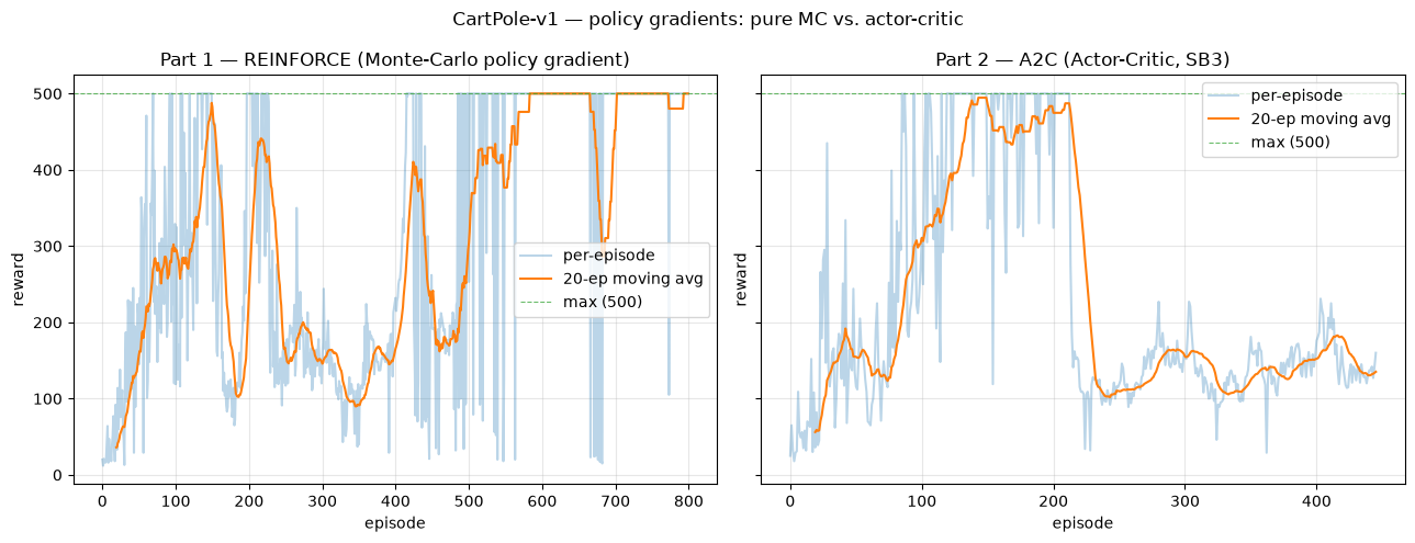
Takeaway: REINFORCE reached ~496 avg return by hand-coding the policy-gradient theorem — increase the log-prob of actions that led to high return-to-go, with a standardised baseline to tame variance. It works, but the curve is jagged: it is an unbiased Monte-Carlo estimate, so it is noisy and needs *whole episodes*. A2C replaces the crude baseline with a learned value **critic** and **bootstraps** off it, so it updates online on short rollouts with far less variance — cleaner, faster, at the cost of a little bias. Its eval score was 145 +/- 7. Next, L6 (PPO) keeps the actor-critic idea but adds a *clipped* objective that stops each update from moving the policy too far — the fix that makes policy gradients robust enough for the real world.