Lesson 4 — Deep Q-Networks: RL’s first real trade

So far our “state” has been a bandit arm — a stateless choice. Trading is not like that. The moment you hold a position, the world you observe next depends on what you did, and the cost of changing your mind is real. That makes trading a genuine Markov Decision Process (MDP), and it is where deep reinforcement learning earns its keep.

In this lesson we point a Deep Q-Network (DQN) — the same algorithm that learned to play Atari from pixels — at common.TradingEnv. DQN learns a Q(state, action) table approximated by a neural net: for each observed market window it estimates the future reward of going short, flat, or long, and picks the best. Experience replay and a slowly-updated target network are what keep that bootstrapped learning stable.

Three ideas do all the teaching here

Position is now part of the state. The observation is the last window log-returns plus the current position. The agent’s own holding feeds back into what it sees, so this is an MDP — not a one-shot signal predictor.
Transaction costs punish churn. Charge a small cost on every change of position and the agent must earn each trade. Remove it and DQN degenerates into flipping long/short every bar — costless noise that any real spread wipes out instantly.
You must evaluate on a HELD-OUT price path. This is the single most important discipline in trading RL. We train on one Ornstein-Uhlenbeck series and test on a different one (a different rng seed). Score the agent on the path it trained on and you are measuring memorisation, not skill.

We use mean-reverting (Ornstein-Uhlenbeck) prices on purpose: there is a real, learnable signal — when price runs above its mean, fade it. On a pure random walk there would be nothing to learn, and honesty demands we not pretend otherwise.

Run order matters. The cells below build on each other. Run them top to bottom (Jupyter: Run → Run All Cells; VS Code: Run All). If you hit NameError (or similar), you skipped the Setup cell — run it first.

Setup — imports & configuration

Run this cell first. It imports every library and defines the module-level constants the rest of the notebook relies on.

import numpy as np
import matplotlib.pyplot as plt
from stable_baselines3 import DQN
from stable_baselines3.common.monitor import Monitor
from stable_baselines3.common.callbacks import BaseCallback
from common import (
    ornstein_uhlenbeck,
    TradingEnv,
    buy_and_hold,
    evaluate_policy_on_env,
    sharpe_ratio,
    max_drawdown,
    plot_learning_curve,
    plot_equity_curves,
    plot_price_and_positions,
)
SEED = 0
TRAIN_SEED = 1
TEST_SEED = 999
N_TRAIN = 6000
N_TEST = 3000
WINDOW = 20
COST = 0.0005
TOTAL_STEPS = 150_000

`RewardLoggerCallback` (class)

Collect per-episode rewards from the Monitor wrapper during training.

Stable-Baselines3’s Monitor writes a summary dict into info["episode"] the moment an episode ends ("r" = total reward, "l" = length). This callback fires on every environment step, watches the infos that SB3 exposes in self.locals, and stashes each finished episode’s reward. That list becomes our learning curve — the honest record of whether training is actually improving the policy, or just burning compute.

class RewardLoggerCallback(BaseCallback):

    def __init__(self):
        super().__init__()
        self.episode_rewards = []

    def _on_step(self):
        for info in self.locals.get("infos", []):
            episode = info.get("episode")
            if episode is not None:
                self.episode_rewards.append(episode["r"])
        return True

`make_prices` (function)

One mean-reverting Ornstein-Uhlenbeck price path from a given seed.

The seed is the whole point of this function: calling it with two different seeds gives two statistically similar but independent markets. We train on one and test on the other, which is the only honest way to ask “did the agent learn a rule, or memorise a path?”.

def make_prices(n, seed):
    rng = np.random.default_rng(seed)
    return ornstein_uhlenbeck(n, rng, mu=1.0, theta=0.05, sigma=0.01)

`train_dqn` (function)

Train a DQN agent on the training environment and log its learning curve.

The hyper-parameters are standard, conservative DQN settings tuned for a small MLP on a dense-reward task:

learning_rate=5e-4 — steady gradient steps on the Q-network.
buffer_size=50_000 with learning_starts=1000 — fill a replay buffer before training so early updates are not dominated by one trajectory.
batch_size=64, train_freq=4 — update every 4 steps on a minibatch.
gamma=0.99 — value future PnL almost as much as present PnL.
target_update_interval=500 — refresh the target network slowly; this is what stops the bootstrapped Q-values from chasing their own tail.
exploration_fraction=0.3 decaying to exploration_final_eps=0.05 — explore aggressively early (ε from 1.0), then mostly exploit.

Returns the trained model and the list of per-episode training rewards.

def train_dqn(train_env, total_steps, seed):
    logger = RewardLoggerCallback()
    model = DQN(
        "MlpPolicy",
        train_env,
        learning_rate=5e-4,
        buffer_size=50_000,
        learning_starts=1000,
        batch_size=64,
        gamma=0.99,
        target_update_interval=500,
        train_freq=4,
        exploration_fraction=0.3,
        exploration_final_eps=0.05,
        device="cpu",
        seed=seed,
        verbose=0,
    )
    model.learn(total_timesteps=total_steps, callback=logger, progress_bar=False)
    return model, logger.episode_rewards

`report_metrics` (function)

Print the three numbers a trader actually judges a strategy by.

def report_metrics(label, metrics):
    print(
        f"{label:14s} | total PnL = {metrics['total_pnl']:+.4f} "
        f"| Sharpe = {metrics['sharpe']:+.2f} "
        f"| max drawdown = {metrics['max_drawdown']:+.4f}"
    )

`main` (function)

def main():
    np.random.seed(SEED)

    # --- Build TRAIN and HELD-OUT TEST markets from DIFFERENT seeds ---------
    train_prices = make_prices(N_TRAIN, TRAIN_SEED)
    test_prices = make_prices(N_TEST, TEST_SEED)
    print(
        f"Train path: {N_TRAIN} bars (seed {TRAIN_SEED}) | "
        f"Held-out test path: {N_TEST} bars (seed {TEST_SEED})"
    )

    # Monitor wraps the training env so episode rewards are logged for the curve.
    train_env = Monitor(TradingEnv(train_prices, window=WINDOW, cost=COST))

    # --- Train ------------------------------------------------------------
    print(f"\nTraining DQN for {TOTAL_STEPS:,} steps on CPU...")
    model, episode_rewards = train_dqn(train_env, TOTAL_STEPS, SEED)
    print(f"Done. Logged {len(episode_rewards)} training episodes.")

    # --- Evaluate on the HELD-OUT test path -------------------------------
    # A fresh env on the test prices: the agent has never seen these returns.
    test_env = TradingEnv(test_prices, window=WINDOW, cost=COST)
    agent = evaluate_policy_on_env(model, test_env, deterministic=True)

    # Buy-and-hold on the SAME held-out env is the baseline to beat.
    bh_env = TradingEnv(test_prices, window=WINDOW, cost=COST)
    bh_pnls = buy_and_hold(bh_env)
    bh_metrics = {
        "total_pnl": float(np.sum(bh_pnls)),
        "sharpe": sharpe_ratio(bh_pnls),
        "max_drawdown": max_drawdown(bh_pnls),
    }

    print("\nHeld-out test performance:")
    report_metrics("DQN agent", agent)
    report_metrics("buy & hold", bh_metrics)

    # --- Figure 1: learning curve -----------------------------------------
    plot_learning_curve(
        episode_rewards, window=10,
        title="DQN training — episode reward over time",
    )
    plt.show()

    # --- Figure 2: equity curves on held-out data -------------------------
    plot_equity_curves(
        {"DQN agent": agent["pnls"], "buy & hold": bh_pnls},
        title="Held-out equity: DQN agent vs buy & hold",
    )
    plt.show()

    # --- Figure 3: what the agent actually did ----------------------------
    plot_price_and_positions(
        test_prices, agent["positions"],
        title="Held-out path — agent position (long/flat/short) vs price",
    )
    plt.show()

    # --- Takeaway ---------------------------------------------------------
    print(
        "\nTakeaway: on mean-reverting data the DQN agent should beat buy & hold "
        "on the HELD-OUT path after costs — it learns to fade extremes rather "
        "than sit long through every dip, so its Sharpe is higher for the risk "
        "it takes. Two honest caveats: (1) this is synthetic, deliberately "
        "tradeable data; real FX has far weaker, non-stationary signal and the "
        "same pipeline will often fail to beat buy & hold there. (2) The only "
        "reason we can trust any of this is that we scored on a DIFFERENT price "
        "path from the one we trained on. Evaluate in-sample and every number "
        "above is a comforting lie."
    )

Run the lesson

Execute everything above, then run main().

main()

Train path: 6000 bars (seed 1) | Held-out test path: 3000 bars (seed 999)

Training DQN for 150,000 steps on CPU...
Done. Logged 25 training episodes.

Held-out test performance:
DQN agent      | total PnL = +1.5482 | Sharpe = +0.82 | max drawdown = -0.2781
buy & hold     | total PnL = -0.0165 | Sharpe = -0.01 | max drawdown = -0.1720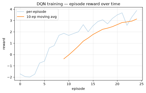


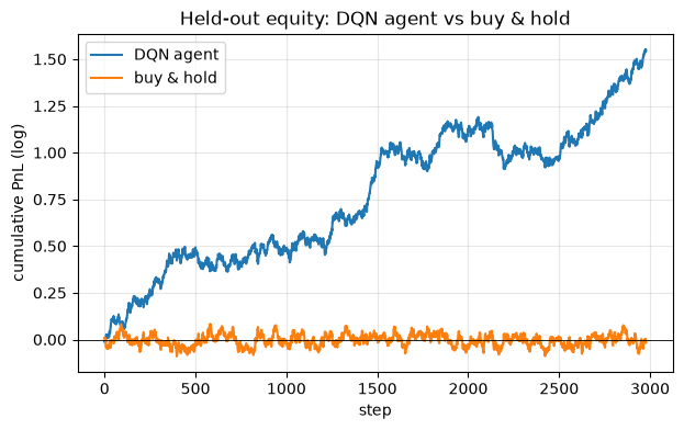
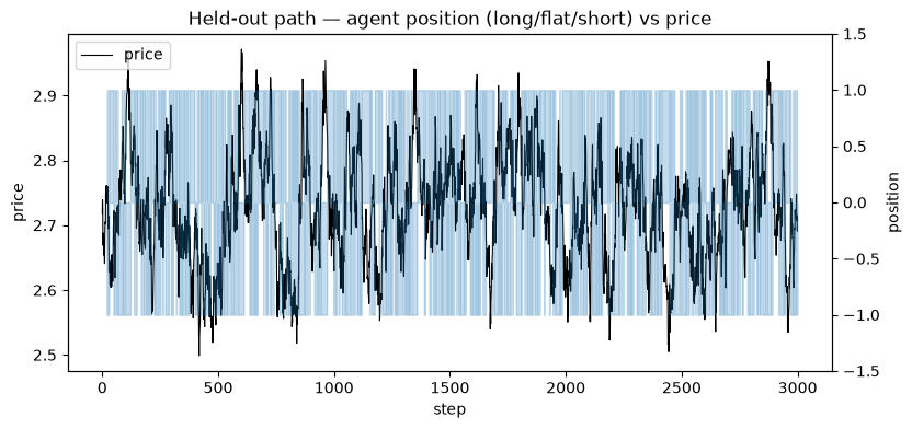
Takeaway: on mean-reverting data the DQN agent should beat buy & hold on the HELD-OUT path after costs — it learns to fade extremes rather than sit long through every dip, so its Sharpe is higher for the risk it takes. Two honest caveats: (1) this is synthetic, deliberately tradeable data; real FX has far weaker, non-stationary signal and the same pipeline will often fail to beat buy & hold there. (2) The only reason we can trust any of this is that we scored on a DIFFERENT price path from the one we trained on. Evaluate in-sample and every number above is a comforting lie.

Three ideas do all the teaching here

Setup — imports & configuration

RewardLoggerCallback (class)

make_prices (function)

train_dqn (function)

report_metrics (function)

main (function)