import numpy as np
import matplotlib.pyplot as plt
import gymnasium as gym
from stable_baselines3 import DQN
from stable_baselines3.common.monitor import Monitor
from stable_baselines3.common.evaluation import evaluate_policy
from stable_baselines3.common.callbacks import BaseCallback
from common import plot_learning_curve
SEED = 0
TOTAL_STEPS = 60000
EVAL_EPISODES = 20Lesson 3 — DQN on CartPole: the first real MDP
In Lessons 1 and 2 the world had no memory. A bandit arm pays you and forgets; the action you take now does not change the problem you face next. That made credit assignment trivial — the reward that arrives is the consequence of the action that just fired.
CartPole breaks that comfort. You push a cart left or right to balance a pole hinged on top of it. The reward is +1 for every timestep the pole stays up, up to 500. But here is the twist that defines reinforcement learning proper:
- the action changes the state (the cart moves, the pole tips),
- that new state is what you must act from next,
- and a bad shove now topples the pole many steps later.
This is delayed reward and the credit-assignment problem. When the pole finally falls, which of the last hundred actions was to blame? A bandit never had to answer that. To answer it we need to reason about future reward, not just the reward in front of us — and that is what a value function does.
Q-learning and the Deep Q-Network
We learn an action-value function Q(s, a): the total future reward we expect if we take action a in state s and act well thereafter. Once we have it, acting is easy — pick argmax_a Q(s, a). The trick is learning it from experience without ever being told the “right” answer.
The engine is bootstrapping via the Bellman equation. The value of a state is the immediate reward plus the (discounted) value of where we land::
Q(s, a) -> r + gamma * max_a' Q(s', a')We nudge our estimate toward that target. The right-hand side uses our own current estimate of the next state — we lift ourselves by our bootstraps. This is the fundamental new machinery versus the bandits: value propagates backward through time, so a reward at step 200 can eventually teach the action at step 100 that it was a mistake.
DQN = Q-learning with a neural network approximating Q, plus two stabilising tricks that make the combination actually work:
- Replay buffer — store transitions
(s, a, r, s')and train on random minibatches drawn from it. Consecutive timesteps are highly correlated (the cart barely moves between frames); shuffling decorrelates the samples so the network does not overfit to whatever it saw in the last few steps. - Target network — a periodically frozen copy of
Qused to compute ther + gamma * max Q(s', a')target. If the target chased the same weights we are updating, we would be aiming at a moving target and training would oscillate or diverge. Freezing it for a while gives a stable goalpost.
Exploration is still the ε-greedy idea from Lesson 1, but now on a schedule: we start acting almost randomly (to fill the buffer with varied experience) and anneal ε down toward greedy as Q becomes trustworthy.
We lean on Stable-Baselines3, a battle-tested implementation, so we can watch the learning dynamics rather than debug gradient math. CartPole-v1 is considered “solved” at an average return around 475 out of 500.
Run order matters. The cells below build on each other. Run them top to bottom (Jupyter: Run → Run All Cells; VS Code: Run All). If you hit
NameError(or similar), you skipped the Setup cell — run it first.
Setup — imports & configuration
Run this cell first. It imports every library and defines the module-level constants the rest of the notebook relies on.
EpisodeRewardCallback (class)
Collect each finished episode’s total reward during training.
Stable-Baselines3 does not hand us a learning curve for free — training interleaves environment steps and gradient updates internally. But because we wrapped the env in a Monitor, every time an episode ends SB3 tucks a summary dict under the "episode" key of that step’s info. This callback fires after every environment step, scans self.locals["infos"] for those end-of-episode markers, and appends the episode return r.
The result, self.episode_rewards, is exactly the raw material for a learning curve: one number per episode, in training order. Watching it climb from ~20 (a flailing random policy) toward ~500 is the whole story of the agent learning to assign credit through time.
class EpisodeRewardCallback(BaseCallback):

    def __init__(self):
        super().__init__()
        self.episode_rewards = []

    def _on_step(self):
        for info in self.locals["infos"]:
            episode = info.get("episode")
            if episode is not None:
                self.episode_rewards.append(episode["r"])
        return True  # returning False would abort training
make_env (function)
Build a single seeded CartPole-v1 environment wrapped in a Monitor.
CartPole-v1 is the classic control MDP: a 4-dimensional continuous state (cart position and velocity, pole angle and angular velocity) and two discrete actions (push left, push right). Reward is +1 per surviving step, capped at 500, so a return near 500 means the pole essentially never fell.
The Monitor wrapper is what makes the environment observable to our callback: it records episode returns and lengths and stamps them into the info dict when each episode terminates. Without it, the "episode" key our callback looks for would never appear.
def make_env():
    env = gym.make("CartPole-v1")
    env = Monitor(env)
    env.reset(seed=SEED)
    return env
train_dqn (function)
Train a Deep Q-Network on the environment and return (model, callback).
Every hyperparameter here maps directly onto a concept from the lesson intro (these are the well-tested values that reliably solve CartPole):
buffer_size=100000/learning_starts=1000— the replay buffer; we collect 1000 transitions of pure experience before any gradient step so the very first minibatches are not degenerate.train_freq=256/gradient_steps=128/batch_size=64— every 256 environment steps we do a burst of 128 gradient updates, each on a decorrelated minibatch of 64 past transitions. Collect a chunk of fresh experience, then replay hard over it.target_update_interval=10— how often the frozen target network is refreshed to the live weights: the stable goalpost for our TD targets.gamma=0.99— the discount that makes future reward count, and hence the reason value can propagate backward and solve credit assignment at all.exploration_fraction=0.16/exploration_final_eps=0.04— the ε-greedy schedule: anneal from fully exploratory down to 4% random over the first 16% of training, then act almost greedily.learning_rate=2.3e-3— step size for the Q-network’s optimiser.net_arch=[256, 256]— the two-hidden-layer MLP approximatingQ.
device="cpu" is deliberate: this is a tiny multilayer perceptron, and for such small networks the overhead of shuttling minibatches to a GPU makes CPU the faster choice (SB3 will warn you about exactly this).
def train_dqn(env):
    model = DQN(
        policy="MlpPolicy",
        env=env,
        learning_rate=2.3e-3,
        buffer_size=100000,
        learning_starts=1000,
        batch_size=64,
        gamma=0.99,
        target_update_interval=10,
        train_freq=256,
        gradient_steps=128,
        exploration_fraction=0.16,
        exploration_final_eps=0.04,
        policy_kwargs=dict(net_arch=[256, 256]),
        seed=SEED,
        device="cpu",
        verbose=0,
    )
    callback = EpisodeRewardCallback()
    model.learn(total_timesteps=TOTAL_STEPS, callback=callback)
    return model, callback
evaluate (function)
Roll the trained, greedy policy out and report mean +/- std return.
Training rewards are noisy — they mix in exploratory (random) actions and a policy that is still improving. To judge the finished agent we turn exploration off (deterministic=True) and average over many fresh episodes. evaluate_policy returns the mean and standard deviation of return across EVAL_EPISODES rollouts; on a solved CartPole this should sit near the 500 ceiling with small spread.
def evaluate(model, env):
    mean_reward, std_reward = evaluate_policy(
        model,
        env,
        n_eval_episodes=EVAL_EPISODES,
        deterministic=True,
    )
    return mean_reward, std_reward
main (function)
def main():
    np.random.seed(SEED)

    env = make_env()
    print(f"Training DQN on CartPole-v1 for {TOTAL_STEPS} steps (CPU, this takes a minute or two)...")
    model, callback = train_dqn(env)

    mean_reward, std_reward = evaluate(model, env)
    print(f"\nEvaluation over {EVAL_EPISODES} greedy episodes: "
          f"mean reward = {mean_reward:.1f} +/- {std_reward:.1f}  (max possible = 500)")

    rewards = np.asarray(callback.episode_rewards)
    print(f"Saw {len(rewards)} training episodes; "
          f"first few returns ~ {rewards[:10].mean():.0f}, "
          f"best training episode = {rewards.max():.0f} "
          f"(the training curve oscillates - DQN is famously wobbly - but the "
          f"final greedy policy above is rock solid).")

    fig, ax = plt.subplots(figsize=(8, 5))
    plot_learning_curve(
        callback.episode_rewards,
        window=20,
        title="DQN on CartPole-v1 — return per training episode",
        ax=ax,
    )
    ax.axhline(475, color="green", ls="--", lw=0.8, label="solved threshold (~475)")
    ax.legend()
    plt.show()

    print(
        "\nTakeaway: unlike the bandits, here the action reshapes the next state, "
        "so a mistake now surfaces as a fallen pole many steps later. DQN cracks "
        "that credit-assignment problem by learning a value function that "
        "bootstraps future reward backward through time (Bellman), while the "
        "replay buffer and target network keep the neural approximation stable. "
        "The learning curve climbing from ~20 to ~500 is value propagation "
        "working: the agent is finally reasoning about consequences, not just "
        "immediate payoff."
    )
Run the lesson
Execute everything above, then run main().
main()Training DQN on CartPole-v1 for 60000 steps (CPU, this takes a minute or two)...
Evaluation over 20 greedy episodes: mean reward = 500.0 +/- 0.0 (max possible = 500)
Saw 643 training episodes; first few returns ~ 22, best training episode = 500 (the training curve oscillates - DQN is famously wobbly - but the final greedy policy above is rock solid).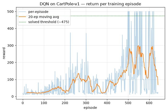
Takeaway: unlike the bandits, here the action reshapes the next state, so a mistake now surfaces as a fallen pole many steps later. DQN cracks that credit-assignment problem by learning a value function that bootstraps future reward backward through time (Bellman), while the replay buffer and target network keep the neural approximation stable. The learning curve climbing from ~20 to ~500 is value propagation working: the agent is finally reasoning about consequences, not just immediate payoff.