import numpy as np
import matplotlib.pyplot as plt
SEED = 0
K = 10
STEPS = 2000
RUNS = 200Lesson 1 — Multi-armed bandits: the honest start for trading
Before we touch a single “state” or “environment step”, we solve the smallest non-trivial decision problem in all of reinforcement learning: the multi-armed bandit. You face k slot machines (arms). Each pays a random reward from an unknown distribution. You have a fixed number of pulls. Which arm do you play?
This is the exploration-vs-exploitation dilemma in its purest form, and it is the honest first model of trading:
- each arm is a strategy (or an asset to allocate to),
- each pull is a period you commit capital,
- the reward is that period’s PnL,
- and you never learn the payoff of a strategy you did not run.
The metric we care about is regret: how much reward we lost versus an oracle who always played the best arm. A good algorithm drives average regret to zero.
We compare four policies, from naive to principled:
- Greedy — always pull the arm with the best average so far. Gets stuck.
- ε-greedy — pull greedily, but with probability ε explore at random.
- UCB — pull the arm with the best optimistic estimate (mean + a bonus that shrinks the more you sample it). “Optimism in the face of uncertainty.”
- Thompson sampling — keep a probability distribution over each arm’s mean and pull the arm that a random draw says is best. Bayesian and remarkably effective.
Run order matters. The cells below build on each other. Run them top to bottom (Jupyter: Run → Run All Cells; VS Code: Run All). If you hit
NameError(or similar), you skipped the Setup cell — run it first.
Setup — imports & configuration
Run this cell first. It imports every library and defines the module-level constants the rest of the notebook relies on.
GaussianBandit (class)
A k-armed bandit with fixed but unknown Gaussian arm means.
Each arm a pays N(mean_a, 1). The means are drawn once from N(0, 1) at construction. pull(a) returns a noisy reward; the agent never sees the true means — only what it earns.
class GaussianBandit:

    def __init__(self, k, rng):
        self.k = k
        self.means = rng.standard_normal(k)
        self.best = self.means.max()
        self.rng = rng

    def pull(self, a):
        return self.means[a] + self.rng.standard_normal()
run_epsilon_greedy (function)
ε-greedy: exploit the best-known arm, but explore at rate epsilon.
We track a running average reward Q[a] per arm (incremental mean, so no need to store history). With probability ε we pull a uniformly random arm; otherwise the current best. ε = 0 is pure greedy — it commits early and often to a wrong arm, which is exactly the failure we want to see.
def run_epsilon_greedy(bandit, steps, epsilon, rng):
    k = bandit.k
    Q = np.zeros(k)
    N = np.zeros(k)
    regret = np.empty(steps)
    for t in range(steps):
        if rng.random() < epsilon:
            a = rng.integers(k)
        else:
            a = int(np.argmax(Q))
        r = bandit.pull(a)
        N[a] += 1
        Q[a] += (r - Q[a]) / N[a]  # incremental sample mean
        regret[t] = bandit.best - bandit.means[a]
    return regret
run_ucb (function)
UCB1: pull argmax(Q[a] + c * sqrt(ln t / N[a])).
The second term is an uncertainty bonus: arms we have sampled little get a large optimistic boost, so they get tried; as N[a] grows the bonus shrinks and we converge on the truly best arm. No randomness needed — the exploration is directed at the least-certain arms. c tunes how bold.
def run_ucb(bandit, steps, c, rng):
    k = bandit.k
    Q = np.zeros(k)
    N = np.zeros(k)
    regret = np.empty(steps)
    for t in range(steps):
        if t < k:
            a = t  # play each arm once to seed the estimates
        else:
            bonus = c * np.sqrt(np.log(t + 1) / N)
            a = int(np.argmax(Q + bonus))
        r = bandit.pull(a)
        N[a] += 1
        Q[a] += (r - Q[a]) / N[a]
        regret[t] = bandit.best - bandit.means[a]
    return regret
run_thompson (function)
Thompson sampling with a Gaussian model of each arm’s mean.
We keep a posterior N(mu[a], 1/N[a]) over each arm’s true mean. Each step we draw one sample per arm from its posterior and pull the arm with the highest sampled value, then update that arm’s posterior with the observed reward. Arms we are unsure about have wide posteriors, so they occasionally win the draw — exploration falls out of the Bayesian maths for free.
def run_thompson(bandit, steps, rng):
    k = bandit.k
    mu = np.zeros(k)
    N = np.ones(k)  # start with a weak prior of one pseudo-observation
    regret = np.empty(steps)
    for t in range(steps):
        sample = mu + rng.standard_normal(k) / np.sqrt(N)
        a = int(np.argmax(sample))
        r = bandit.pull(a)
        N[a] += 1
        mu[a] += (r - mu[a]) / N[a]
        regret[t] = bandit.best - bandit.means[a]
    return regret
average_cumulative_regret (function)
Average cumulative regret across many independent bandits.
A single bandit run is noisy — one lucky/unlucky seed tells you little. We average over runs fresh bandits (each with new arm means) so the curves reflect the policy, not one draw. Cumulative regret that flattens means the policy has found and stuck to the best arm.
def average_cumulative_regret(policy_fn, runs, steps):
    total = np.zeros(steps)
    for r in range(runs):
        rng = np.random.default_rng(SEED + r)
        bandit = GaussianBandit(K, rng)
        total += np.cumsum(policy_fn(bandit, steps, rng))
    return total / runs
main (function)
def main():
    # Each policy is a thunk taking (bandit, steps, rng); average its regret.
    policies = {
        "greedy (ε=0)":        lambda b, s, rng: run_epsilon_greedy(b, s, 0.0, rng),
        "ε-greedy (ε=0.1)":    lambda b, s, rng: run_epsilon_greedy(b, s, 0.1, rng),
        "UCB (c=2)":           lambda b, s, rng: run_ucb(b, s, 2.0, rng),
        "Thompson sampling":   lambda b, s, rng: run_thompson(b, s, rng),
    }

    fig, ax = plt.subplots(figsize=(8, 5))
    for name, fn in policies.items():
        curve = average_cumulative_regret(fn, RUNS, STEPS)
        ax.plot(curve, label=name)
        print(f"{name:22s} final cumulative regret = {curve[-1]:7.1f}")
    ax.set_xlabel("pull")
    ax.set_ylabel("cumulative regret (avg over runs)")
    ax.set_title(f"{K}-armed Gaussian bandit — lower & flatter is better")
    ax.legend()
    ax.grid(alpha=0.3)
    plt.show()

    print(
        "\nTakeaway: greedy plateaus with high regret (it commits to a wrong arm "
        "and never revisits). ε-greedy keeps exploring forever, so its regret "
        "grows linearly — just slowly. UCB and Thompson drive *marginal* regret "
        "toward zero: their curves bend flat. That directed-exploration instinct "
        "is what we carry into every RL algorithm that follows."
    )
Run the lesson
Execute everything above, then run main().
main()greedy (ε=0) final cumulative regret = 989.1
ε-greedy (ε=0.1) final cumulative regret = 392.2
UCB (c=2) final cumulative regret = 187.7
Thompson sampling final cumulative regret = 78.3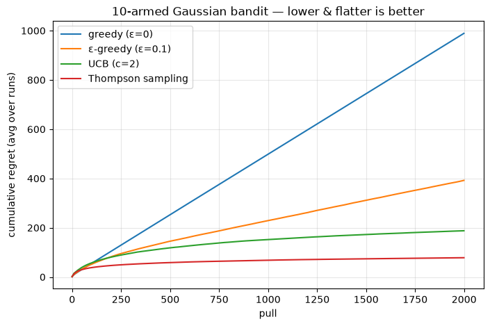
Takeaway: greedy plateaus with high regret (it commits to a wrong arm and never revisits). ε-greedy keeps exploring forever, so its regret grows linearly — just slowly. UCB and Thompson drive *marginal* regret toward zero: their curves bend flat. That directed-exploration instinct is what we carry into every RL algorithm that follows.