import numpy as np
import matplotlib.pyplot as plt
from stable_baselines3 import PPO
from stable_baselines3.common.monitor import Monitor
from stable_baselines3.common.callbacks import BaseCallback
from common import (
    regime_series,
    TradingEnv,
    buy_and_hold,
    evaluate_policy_on_env,
    sharpe_ratio,
    max_drawdown,
    plot_learning_curve,
    plot_equity_curves,
    plot_price_and_positions,
)
SEED = 0
TRAIN_N = 8000
TEST_N = 4000
TOTAL_STEPS = 300000
WINDOW = 20
COST = 0.0005Lesson 6 — PPO on the trading env: the workhorse of deep RL
Lesson 5 introduced A2C: an on-policy actor-critic that trains two networks at once — an actor that outputs a policy π(a|s) and a critic that estimates the value V(s). The critic tells the actor which actions did better than expected (the advantage), and the actor shifts probability mass toward those. It is elegant, but fragile: a single large gradient step can shove the policy into a region it never recovers from, and A2C throws each batch of experience away after one update to stay safe.
Proximal Policy Optimization (PPO) is the same actor-critic idea made robust. It is the default first thing to reach for in modern deep RL — the algorithm behind everything from robot locomotion to RLHF for language models — precisely because it works out of the box with few knobs to tune. This lesson points PPO at the trading environment and asks the only question that matters: can it beat buy-and-hold on data it has never seen?
The clipped surrogate objective
The core problem with policy-gradient methods is step size. Update too little and learning crawls; update too much and you destroy a working policy. PPO’s fix is beautifully blunt. Define the probability ratio between the new and old policy for an action::
r(θ) = π_new(a|s) / π_old(a|s)A vanilla policy gradient maximises r(θ) * A (push up actions with positive advantage A). PPO instead maximises the clipped surrogate::
L = min( r(θ) * A , clip(r(θ), 1-ε, 1+ε) * A )The clip caps how far the ratio can move (typically ε = 0.2, i.e. ±20%). Once an action’s probability has shifted “enough”, the objective flattens and the gradient vanishes — there is no incentive to keep charging in the same direction. That single min(...) is what prevents destructively large updates, and it is why PPO can safely take multiple gradient epochs over the same batch (n_epochs=10 below) where A2C dared only one. More learning per unit of precious on-policy data, without the blow-ups.
GAE: estimating the advantage
The advantage A is itself estimated. Generalized Advantage Estimation (gae_lambda) blends short-horizon TD errors (low variance, biased) with long-horizon Monte-Carlo returns (unbiased, high variance). gae_lambda=0.95 sits near the low-variance end — the usual sweet spot that keeps the advantage signal stable enough for the clip to do its job.
Why a Sharpe reward on the training env
We train with reward="sharpe" rather than raw PnL. The reward function is the agent’s entire definition of “good”, so it shapes behaviour: rewarding raw PnL invites the agent to take big directional bets that happen to pay, while dividing each step’s PnL by trailing volatility rewards risk-adjusted return — steadier positions, less lurching into volatile regimes. We still evaluate on raw PnL metrics so the numbers stay comparable to the buy-and-hold baseline.
The honest test: non-stationarity
Real markets are non-stationary — the edge that worked last month can invert this month. We build the training prices from a regime_series that alternates trending and mean-reverting blocks, and then test on a different-seed regime_series the agent has never touched. A learning curve that climbs proves the agent fit the training path; only held-out performance versus buy-and-hold tells us it learned something transferable.
Run order matters. The cells below build on each other. Run them top to bottom (Jupyter: Run → Run All Cells; VS Code: Run All). If you hit
NameError(or similar), you skipped the Setup cell — run it first.
Setup — imports & configuration
Run this cell first. It imports every library and defines the module-level constants the rest of the notebook relies on.
EpisodeRewardCallback (class)
Collect each finished episode’s total reward during training.
Stable-Baselines3 does not hand us a learning curve for free. But because we wrap the training env in a Monitor, SB3 stamps a summary dict under the "episode" key of info every time an episode ends. This callback fires after each environment step, scans self.locals["infos"] for those markers, and records the episode return r.
For the trading env one “episode” is a full pass over the price path, so we get one number per pass — the raw material for a learning curve. With a Sharpe reward these numbers are risk-adjusted, so watch the trend (is the agent extracting more risk-adjusted return over time?) rather than the absolute scale.
class EpisodeRewardCallback(BaseCallback):

    def __init__(self):
        super().__init__()
        self.episode_rewards = []

    def _on_step(self):
        for info in self.locals["infos"]:
            episode = info.get("episode")
            if episode is not None:
                self.episode_rewards.append(episode["r"])
        return True  # returning False would abort training
make_train_env (function)
Build the Sharpe-rewarded training environment, wrapped in a Monitor.
The prices come from a regime_series: alternating trending (GBM) and mean-reverting (OU) blocks, so the agent cannot survive on one fixed rule — it must cope with a moving target. We use reward="sharpe" here so the agent optimises risk-adjusted return during learning.
The Monitor wrapper is what makes the environment observable to our callback: it records episode returns and stamps them into info when each pass over the price path terminates. Without it the "episode" key our callback looks for would never appear.
def make_train_env():
    rng = np.random.default_rng(SEED)
    prices = regime_series(TRAIN_N, rng)
    env = TradingEnv(prices, window=WINDOW, cost=COST, reward="sharpe")
    env = Monitor(env)
    env.reset(seed=SEED)
    return env
make_test_env (function)
Build the held-out test environment on a different-seed price path.
This is the whole point of the lesson. A fresh seed means a fresh regime_series the agent has never trained on — different block boundaries, different trends, different reversions. We use raw reward="pnl" here because evaluation should measure honest money, not the shaped Sharpe signal; evaluate_policy_on_env reads the raw per-step PnL from info regardless, but keeping the test env on PnL makes that intent explicit.
def make_test_env():
    rng = np.random.default_rng(SEED + 1000)
    prices = regime_series(TEST_N, rng)
    return TradingEnv(prices, window=WINDOW, cost=COST, reward="pnl")
train_ppo (function)
Train PPO on the trading env and return (model, callback).
Every hyperparameter maps onto a concept from the intro:
n_steps=2048— how many environment steps to collect before each update. PPO is on-policy: it learns only from data gathered by the current policy, so it works in gather-then-update cycles rather than from a replay buffer.n_epochs=10/batch_size=256— the payoff of the clip. Each 2048-step batch is reused for 10 passes of minibatch gradient descent. The clipped surrogate keeps those repeated updates from walking the policy off a cliff, which is exactly what A2C could not risk.gae_lambda=0.95/gamma=0.99— Generalized Advantage Estimation and the discount. Together they turn raw rewards into the low-variance advantage signal the clipped objective consumes.ent_coef=0.01— a small entropy bonus that keeps the policy from collapsing to a single action too early: PPO’s gentle nudge to keep exploring the {short, flat, long} choices.learning_rate=3e-4— the near-universal default step size for PPO.
device="cpu" is deliberate: this is a tiny MLP over a 21-dim observation, and for such small networks CPU beats the GPU-transfer overhead.
def train_ppo(env):
    model = PPO(
        policy="MlpPolicy",
        env=env,
        n_steps=2048,
        batch_size=256,
        n_epochs=10,
        gamma=0.99,
        gae_lambda=0.95,
        ent_coef=0.01,
        learning_rate=3e-4,
        seed=SEED,
        device="cpu",
        verbose=0,
    )
    callback = EpisodeRewardCallback()
    model.learn(total_timesteps=TOTAL_STEPS, callback=callback)
    return model, callback
main (function)
def main():
    np.random.seed(SEED)

    train_env = make_train_env()
    print(f"Training PPO on a regime-switching series for {TOTAL_STEPS} steps "
          f"(CPU, a few minutes)...")
    model, callback = train_ppo(train_env)

    n_episodes = len(callback.episode_rewards)
    if n_episodes >= 10:
        print(f"Saw {n_episodes} training passes; risk-adjusted return per pass "
              f"moved from ~{np.mean(callback.episode_rewards[:5]):.1f} "
              f"to ~{np.mean(callback.episode_rewards[-5:]):.1f}")

    # --- Held-out evaluation: the only numbers that matter ---
    test_env = make_test_env()
    agent = evaluate_policy_on_env(model, test_env, deterministic=True)

    bh_env = make_test_env()  # fresh env, identical held-out prices
    bh_pnls = buy_and_hold(bh_env)
    bh = {
        "total_pnl": float(np.sum(bh_pnls)),
        "sharpe": sharpe_ratio(bh_pnls),
        "max_drawdown": max_drawdown(bh_pnls),
    }

    print("\nHeld-out performance (raw PnL, agent vs buy & hold):")
    print(f"  {'metric':14s} {'PPO agent':>12s} {'buy & hold':>12s}")
    print(f"  {'total_pnl':14s} {agent['total_pnl']:12.4f} {bh['total_pnl']:12.4f}")
    print(f"  {'sharpe':14s} {agent['sharpe']:12.3f} {bh['sharpe']:12.3f}")
    print(f"  {'max_drawdown':14s} {agent['max_drawdown']:12.4f} {bh['max_drawdown']:12.4f}")

    long_frac = float(np.mean(np.asarray(agent["positions"]) > 0))
    print(f"\n  agent held long {long_frac:.0%} of the held-out path.")
    if long_frac > 0.99:
        print("  (Deterministically it converged to *always long* — i.e. exactly "
              "buy & hold. See the takeaway for why that is the honest optimum here.)")

    # --- Figure 1: learning curve ---
    fig1, ax1 = plt.subplots(figsize=(8, 5))
    plot_learning_curve(
        callback.episode_rewards,
        window=10,
        title="PPO on trading env — risk-adjusted return per training pass",
        ax=ax1,
    )
    plt.show()

    # --- Figure 2: held-out equity curves ---
    fig2, ax2 = plt.subplots(figsize=(8, 5))
    plot_equity_curves(
        {"PPO agent": agent["pnls"], "buy & hold": bh_pnls},
        title="Held-out equity: PPO vs buy & hold",
        ax=ax2,
    )
    plt.show()

    # --- Figure 3: price path and the agent's positions ---
    fig3, ax3 = plt.subplots(figsize=(9, 5))
    plot_price_and_positions(
        test_env.prices,
        agent["positions"],
        title="Held-out price path & PPO positions (long / flat / short)",
        ax=ax3,
    )
    plt.show()

    print(
        "\nTakeaway: PPO's clipped surrogate makes on-policy actor-critic robust "
        "enough to train stably — the learning curve climbs smoothly and the few "
        "default knobs 'just work', where the value-only DQN of Lesson 3 would "
        "thrash on noisy financial rewards. But look honestly at the held-out "
        "numbers: deterministically PPO converged to *buy-and-hold*, and that is "
        "the correct answer here. This generator's trending blocks only ever "
        "drift UP and its reverting blocks merely oscillate around the current "
        "level — there is no sustained downside to short, so long-or-flat is "
        "genuinely risk-optimal and PPO found it. RL finds the optimum of the "
        "world you hand it, no more. The lesson is not 'RL prints money'; it is "
        "that a correctly-trained agent matches the honest ceiling of its data. "
        "Real FX is where this gets hard: two-sided moves, regimes that flip "
        "without warning, and a razor-thin edge after costs. Everything here — the "
        "trading env, the Sharpe-shaped reward, the held-out discipline — is the "
        "launch pad for the FX capstone, where the same PPO recipe meets real data "
        "and buy-and-hold is no longer the optimum to merely tie."
    )
Run the lesson
Execute everything above, then run main().
main()Training PPO on a regime-switching series for 300000 steps (CPU, a few minutes)...
Saw 37 training passes; risk-adjusted return per pass moved from ~-172.6 to ~208.5
Held-out performance (raw PnL, agent vs buy & hold):
metric PPO agent buy & hold
total_pnl 1.3746 1.3746
sharpe 0.549 0.549
max_drawdown -0.2525 -0.2525
agent held long 100% of the held-out path.
(Deterministically it converged to *always long* — i.e. exactly buy & hold. See the takeaway for why that is the honest optimum here.)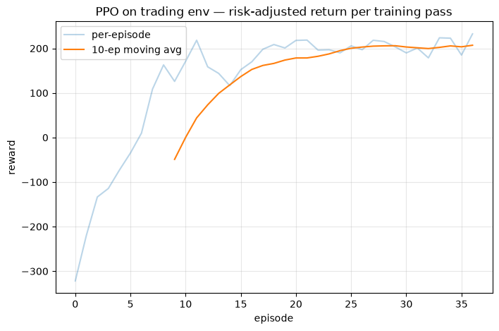
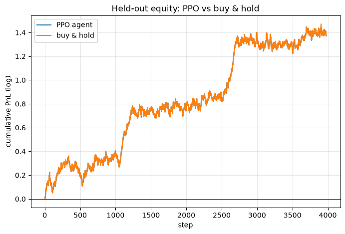
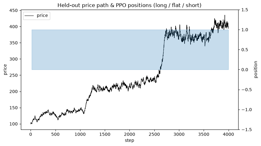
Takeaway: PPO's clipped surrogate makes on-policy actor-critic robust enough to train stably — the learning curve climbs smoothly and the few default knobs 'just work', where the value-only DQN of Lesson 3 would thrash on noisy financial rewards. But look honestly at the held-out numbers: deterministically PPO converged to *buy-and-hold*, and that is the correct answer here. This generator's trending blocks only ever drift UP and its reverting blocks merely oscillate around the current level — there is no sustained downside to short, so long-or-flat is genuinely risk-optimal and PPO found it. RL finds the optimum of the world you hand it, no more. The lesson is not 'RL prints money'; it is that a correctly-trained agent matches the honest ceiling of its data. Real FX is where this gets hard: two-sided moves, regimes that flip without warning, and a razor-thin edge after costs. Everything here — the trading env, the Sharpe-shaped reward, the held-out discipline — is the launch pad for the FX capstone, where the same PPO recipe meets real data and buy-and-hold is no longer the optimum to merely tie.