import numpy as np
import matplotlib.pyplot as plt
SEED = 0
N_ARMS = 3
DIM = 6
STEPS = 2000
RUNS = 200
ALPHA = 1.0
EPSILON = 0.1
RIDGE = 1.0Lesson 2 — Contextual bandits: the bridge from bandits to trading
In Lesson 1 the arms were fixed: the best slot machine was the best on every pull, forever. Real markets are not like that. The right trade depends on what you see — momentum, volatility, order-flow imbalance. The contextual bandit adds exactly one thing to L1’s bandit, and it is the thing that makes the model honest: a state.
Each step you now:
- observe a context vector
x(the market features right now), - choose an arm (an action),
- collect a reward that depends on both
xand the arm.
This is the honest first model of a trading signal:
- context = features — whatever your model gets to look at,
- action = the trade — here
{short, flat, long}, - reward = one-step PnL — how that action paid off given those features.
The one crucial caveat that keeps this a bandit and not yet a full RL problem: there is NO inventory. Your action does not change the context you see next step — contexts arrive i.i.d. from the market, indifferent to what you did. You never carry a position forward, so there is no state dynamics to plan around. That is the whole difference between a bandit and an MDP; Lesson 3 adds the state dynamics (inventory, transaction costs, path-dependence) and turns this into real trading.
Because the reward is linear in the features here, we can be principled. We compare three policies:
- Random — pick an arm uniformly. The do-nothing baseline.
- ε-greedy linear — fit a ridge-regression estimate of each arm’s reward as a function of
x; act greedily on the predictions, explore with prob ε. - LinUCB — the contextual heir of UCB1 from L1. Predict each arm’s reward and an uncertainty bonus that shrinks as you gather data in each direction of feature space; play the most optimistic arm. Directed exploration wins.
Run order matters. The cells below build on each other. Run them top to bottom (Jupyter: Run → Run All Cells; VS Code: Run All). If you hit
NameError(or similar), you skipped the Setup cell — run it first.
Setup — imports & configuration
Run this cell first. It imports every library and defines the module-level constants the rest of the notebook relies on.
LinearContextualBandit (class)
A contextual bandit whose reward is linear in the context features.
Each arm a owns an unknown weight vector w_a (drawn once from N(0, I)). At every step a fresh context x ~ N(0, I) arrives, and the reward for playing arm a is x · w_a + noise. Crucially, x is drawn independently of the agent’s past actions — your trade does not move the market you see next. That i.i.d. context is what makes this a bandit.
Read it as trading: x are today’s features, w_a is how arm a’s one-step PnL loads on each feature, and the oracle is whoever always picks argmax_a x · w_a — the best trade given what is visible.
class LinearContextualBandit:

    def __init__(self, n_arms, dim, rng):
        self.n_arms = n_arms
        self.dim = dim
        self.rng = rng
        self.W = rng.standard_normal((n_arms, dim))  # true per-arm weights
        self.noise = 0.1

    def context(self):
        return self.rng.standard_normal(self.dim)

    def reward(self, x, a):
        return float(x @ self.W[a] + self.noise * self.rng.standard_normal())

    def expected(self, x, a):
        """Noise-free expected reward — used only to score regret, never seen."""
        return float(x @ self.W[a])

    def best_expected(self, x):
        return float((self.W @ x).max())
run_random (function)
Random policy: ignore the context, pick an arm uniformly.
This never learns and never exploits the features, so its per-step regret stays flat and positive: cumulative regret grows in a straight line. It is the “why bother with a model” line every other curve must beat.
def run_random(bandit, steps, rng):
    regret = np.empty(steps)
    for t in range(steps):
        x = bandit.context()
        a = int(rng.integers(bandit.n_arms))
        bandit.reward(x, a)  # collected, but unused — nothing to learn
        regret[t] = bandit.best_expected(x) - bandit.expected(x, a)
    return regret
run_epsilon_greedy_linear (function)
ε-greedy over per-arm ridge-regression predictions of the reward.
For each arm we keep the ridge sufficient statistics A = ridge*I + Σ x xᵀ and b = Σ r x. The least-squares (MAP) weight estimate is θ_a = A_a⁻¹ b_a, so the predicted reward of arm a in context x is θ_a · x. We act greedily on those predictions, but with probability ε we pull a uniformly random arm to keep gathering data on every arm.
This is a genuinely good baseline — it uses the features — but its exploration is undirected: the ε pulls are scattered blindly, wasting samples on arms and directions it is already sure about.
def run_epsilon_greedy_linear(bandit, steps, epsilon, ridge, rng):
    n, d = bandit.n_arms, bandit.dim
    A = np.array([ridge * np.eye(d) for _ in range(n)])
    b = np.zeros((n, d))
    regret = np.empty(steps)
    for t in range(steps):
        x = bandit.context()
        if rng.random() < epsilon:
            a = int(rng.integers(n))
        else:
            theta = np.array([np.linalg.solve(A[i], b[i]) for i in range(n)])
            a = int(np.argmax(theta @ x))
        r = bandit.reward(x, a)
        A[a] += np.outer(x, x)
        b[a] += r * x
        regret[t] = bandit.best_expected(x) - bandit.expected(x, a)
    return regret
run_linucb (function)
LinUCB (disjoint linear model): UCB1’s contextual heir.
Same ridge statistics per arm — A_a and b_a — giving the point estimate θ_a = A_a⁻¹ b_a. But instead of trusting θ_a · x blindly we add an optimism bonus::
p_a = θ_a · x + alpha * sqrt( x · A_a⁻¹ · x )The bonus is large when x points in a direction of feature space this arm has seen little of (A_a⁻¹ still big there), and shrinks as evidence accumulates — the exact contextual analogue of UCB1’s sqrt(ln t / N). We play argmax_a p_a: optimism in the face of uncertainty, now aimed at the least-certain directions, not just the least-pulled arms. alpha tunes how bold. This directed exploration is why LinUCB should clearly win.
def run_linucb(bandit, steps, alpha, ridge, rng):
    n, d = bandit.n_arms, bandit.dim
    A = np.array([ridge * np.eye(d) for _ in range(n)])
    b = np.zeros((n, d))
    regret = np.empty(steps)
    for t in range(steps):
        x = bandit.context()
        p = np.empty(n)
        for i in range(n):
            A_inv = np.linalg.inv(A[i])
            theta = A_inv @ b[i]
            p[i] = theta @ x + alpha * np.sqrt(x @ A_inv @ x)
        a = int(np.argmax(p))
        r = bandit.reward(x, a)
        A[a] += np.outer(x, x)
        b[a] += r * x
        regret[t] = bandit.best_expected(x) - bandit.expected(x, a)
    return regret
average_cumulative_regret (function)
Average cumulative regret across many independent contextual bandits.
Exactly the L1 idea, one dimension richer. A single run is noisy, so we average over runs fresh bandits — each with new arm weights w_a and a new stream of contexts — so the curves reflect the policy, not one draw. Regret at each step is max_a (x·w_a) - x·w_chosen (how much expected PnL we left on the table given the features). A curve that bends flat means the policy has learned to read the context and stopped losing to the oracle.
def average_cumulative_regret(policy_fn, runs, steps):
    total = np.zeros(steps)
    for r in range(runs):
        rng = np.random.default_rng(SEED + r)
        bandit = LinearContextualBandit(N_ARMS, DIM, rng)
        total += np.cumsum(policy_fn(bandit, steps, rng))
    return total / runs
main (function)
def main():
    # Each policy is a thunk taking (bandit, steps, rng); average its regret.
    policies = {
        "random":               lambda b, s, rng: run_random(b, s, rng),
        "ε-greedy linear":      lambda b, s, rng: run_epsilon_greedy_linear(b, s, EPSILON, RIDGE, rng),
        "LinUCB":               lambda b, s, rng: run_linucb(b, s, ALPHA, RIDGE, rng),
    }

    fig, ax = plt.subplots(figsize=(8, 5))
    finals = {}
    for name, fn in policies.items():
        curve = average_cumulative_regret(fn, RUNS, STEPS)
        finals[name] = curve[-1]
        ax.plot(curve, label=name)
        print(f"{name:18s} final cumulative regret = {curve[-1]:7.1f}")
    ax.set_xlabel("decision step")
    ax.set_ylabel("cumulative regret (avg over runs)")
    ax.set_title(f"{N_ARMS}-arm linear contextual bandit — lower & flatter is better")
    ax.legend()
    ax.grid(alpha=0.3)
    plt.show()

    print(
        "\nTakeaway: random ignores the features, so its regret climbs in a "
        "straight line — the market is talking and it isn't listening. ε-greedy "
        "linear *does* use the features and learns fast, but its blind ε-pulls "
        "leak regret forever. LinUCB explores where it is uncertain and nowhere "
        "else, so its curve bends flattest and its final regret is lowest. "
        "\n\nThe leap from L1: reward now depends on a context x — that is a "
        "trading signal (features -> trade -> one-step PnL). But your action "
        "never changes the next x: no inventory, no dynamics, so this is still a "
        "bandit. L3 adds the state dynamics and makes it a real MDP."
    )
Run the lesson
Execute everything above, then run main().
main()random final cumulative regret = 3999.8
ε-greedy linear final cumulative regret = 422.6
LinUCB final cumulative regret = 19.6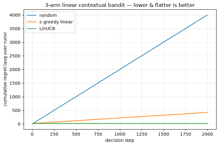
Takeaway: random ignores the features, so its regret climbs in a straight line — the market is talking and it isn't listening. ε-greedy linear *does* use the features and learns fast, but its blind ε-pulls leak regret forever. LinUCB explores where it is uncertain and nowhere else, so its curve bends flattest and its final regret is lowest.

The leap from L1: reward now depends on a context x — that is a trading signal (features -> trade -> one-step PnL). But your action never changes the next x: no inventory, no dynamics, so this is still a bandit. L3 adds the state dynamics and makes it a real MDP.