import numpy as np
import matplotlib.pyplot as plt
from stable_baselines3 import PPO
from stable_baselines3.common.monitor import Monitor
from stable_baselines3.common.callbacks import BaseCallback
from common.fx_toxic_flow import ToxicFlowMarketMakingEnv, avellaneda_stoikov_policy
from common import sharpe_ratio, plot_learning_curve
SEED = 0
TOXICITY = 0.7
N_TRAIN = 6000
N_TEST = 4000
TOTAL_STEPS = 300_000Capstone L2 — Toxic flow: where Avellaneda-Stoikov breaks
The first capstone lived in the Avellaneda-Stoikov world: independent Poisson RFQs, a driftless mid, one dealer. There, PPO learned to skew like the closed form and matched it. This lesson breaks the three assumptions that hurt most in real FX, and watches the closed form get run over.
The three frictions we add
- Clustered arrivals (Hawkes). Each fill raises the intensity of further fills, so flow arrives in bursts — you get loaded before you can re-quote.
- Correlated, simultaneous multi-client fills. Inside a burst, clients trade the same way (a shared latent flow direction). You can be taken out by several at once, all on one side — the scenario A-S structurally cannot represent.
- Adverse selection. The reason everyone sells to you at once is that the mid is about to drop. After fills, the mid drifts against the inventory you were left holding. Winning big one-sided flow is a trap, not a profit.
Because you cannot re-quote inside a burst, the agent also gets a hedge action: dump inventory into the market at a cost. A-S has no such lever.
Why this is the whole point
A-S is optimal for its world — but its world assumes uninformed flow. Drop that assumption and the q·γσ² skew keeps happily quoting into toxic flow, accumulating exactly the inventory that is about to lose. A learned policy sees the burst intensity and the signed flow imbalance in its state — information the static formula integrates away — and can widen, skew, and hedge before the damage. That extra state is the edge.
We train PPO on the toxic-flow env and judge it on a held-out market against the closed-form Avellaneda-Stoikov policy. The bar is not “make money” — under adverse selection that is hard — it is lose far less by managing the toxicity A-S ignores.
Run order matters. The cells below build on each other. Run them top to bottom (Jupyter: Run → Run All Cells; VS Code: Run All). If you hit
NameError(or similar), you skipped the Setup cell — run it first.
Setup — imports & configuration
Run this cell first. It imports every library and defines the module-level constants the rest of the notebook relies on.
make_env (function)
Build a toxic-flow market from a given market seed.
A different seed_market gives a different price path, burst timing, and flow direction — a genuinely held-out test of whether the policy learned to manage toxicity or just memorised one path.
def make_env(seed_market, n):
    return ToxicFlowMarketMakingEnv(n_steps=n, seed_market=seed_market, toxicity=TOXICITY)
rollout (function)
Run one full pass and collect everything needed to score and visualise.
Returns per-step economic PnL (spread + mark-to-market − hedge), the inventory path, arrival intensity, and the running spread / adverse / hedge tallies — so we can show not just that A-S loses but why (its inventory swings load up right into the adverse drift).
def rollout(env, act_fn):
    obs, _ = env.reset()
    pnls, inv, intensity = [], [], []
    done = False
    while not done:
        obs, reward, term, trunc, info = env.step(act_fn(env, obs))
        pnls.append(info["step_pnl"])
        inv.append(info["inventory"])
        intensity.append(info["intensity"])
        done = term or trunc
    return {
        "pnls": pnls, "inventory": inv, "intensity": intensity,
        "net_pnl": float(env.spread_pnl + env.adverse_pnl - env.hedge_cost_paid),
        "spread": float(env.spread_pnl), "adverse": float(env.adverse_pnl),
        "hedge": float(env.hedge_cost_paid), "n_fills": env.fills,
        "inv_std_m": float(np.std(inv)) / 1e6, "sharpe": sharpe_ratio(pnls),
    }
LearningCurve (class)
Log each training episode’s reward for the learning-curve plot.
class LearningCurve(BaseCallback):

    def __init__(self):
        super().__init__()
        self.rewards = []

    def _on_step(self):
        for info in self.locals.get("infos", []):
            ep = info.get("episode")
            if ep is not None:
                self.rewards.append(ep["r"])
        return True
train_ppo (function)
Train PPO on the toxic-flow env.
The reward is dominated by noisy inventory mark-to-market, so we lean on PPO’s stability (clipped updates, GAE) and a slightly larger rollout to average over many bursts per update.
def train_ppo(train_env, total_steps):
    model = PPO("MlpPolicy", train_env, seed=SEED, device="cpu", verbose=0,
                n_steps=4096, batch_size=256, gae_lambda=0.95, gamma=0.99,
                ent_coef=0.01, learning_rate=3e-4, n_epochs=10)
    cb = LearningCurve()
    model.learn(total_timesteps=total_steps, callback=cb, progress_bar=False)
    return model, cb.rewards
main (function)
def main():
    train_env = Monitor(make_env(SEED, N_TRAIN))
    print(f"Training PPO on toxic flow (toxicity={TOXICITY}) for {TOTAL_STEPS:,} steps...")
    model, curve = train_ppo(train_env, TOTAL_STEPS)

    test_env = make_env(SEED + 999, N_TEST)

    def ppo_act(env, obs):
        action, _ = model.predict(obs, deterministic=True)
        return action

    results = {
        "PPO (learned)":       rollout(test_env, ppo_act),
        "Avellaneda–Stoikov":  rollout(test_env, lambda e, o: avellaneda_stoikov_policy(e, 1.2)),
    }

    print("\nHeld-out performance under toxic flow")
    print(f"{'policy':22s}{'net PnL':>11s}{'spread':>10s}{'adverse':>11s}"
          f"{'hedge':>9s}{'inv std':>9s}{'fills':>7s}")
    for name, r in results.items():
        print(f"{name:22s}{r['net_pnl']:>11,.0f}{r['spread']:>10,.0f}"
              f"{r['adverse']:>11,.0f}{r['hedge']:>9,.0f}{r['inv_std_m']:>8.1f}M{r['n_fills']:>7d}")

    # --- plots ---------------------------------------------------------------
    fig, axes = plt.subplots(2, 2, figsize=(13, 9))
    plot_learning_curve(curve, window=20, title="PPO learning curve (episode reward)", ax=axes[0, 0])

    ax = axes[0, 1]
    for name, r in results.items():
        ax.plot(np.cumsum(r["pnls"]) / 1e3, label=name)
    ax.axhline(0, color="k", lw=0.6)
    ax.set_title("Cumulative PnL, held-out ($k)")
    ax.set_xlabel("step"); ax.set_ylabel("cum PnL ($k)"); ax.legend(); ax.grid(alpha=0.3)

    ax = axes[1, 0]
    for name, r in results.items():
        ax.plot(np.asarray(r["inventory"]) / 1e6, label=name, lw=0.8)
    ax.axhline(0, color="k", lw=0.6)
    ax.set_title("Inventory path — A-S loads up into toxic flow; PPO stays flat")
    ax.set_xlabel("step"); ax.set_ylabel("inventory (M units)"); ax.legend(); ax.grid(alpha=0.3)

    # PnL decomposition: how the net number is built (spread vs adverse vs hedge)
    ax = axes[1, 1]
    labels = list(results.keys())
    spread = [results[k]["spread"] / 1e3 for k in labels]
    adverse = [results[k]["adverse"] / 1e3 for k in labels]
    hedge = [-results[k]["hedge"] / 1e3 for k in labels]
    x = np.arange(len(labels))
    ax.bar(x, spread, 0.5, label="spread earned", color="tab:green")
    ax.bar(x, adverse, 0.5, bottom=spread, label="adverse selection", color="tab:red")
    ax.bar(x, hedge, 0.5, bottom=np.array(spread) + np.array(adverse), label="hedge cost", color="tab:orange")
    ax.axhline(0, color="k", lw=0.8)
    ax.set_xticks(x); ax.set_xticklabels(labels, fontsize=9)
    ax.set_title("PnL decomposition ($k)"); ax.set_ylabel("$k"); ax.legend()

    plt.tight_layout(); plt.show()

    ppo, as_ = results["PPO (learned)"], results["Avellaneda–Stoikov"]
    print(
        f"\nTakeaway: Avellaneda–Stoikov assumes uninformed flow, so it keeps "
        f"quoting into the bursts and loads up to an inventory std of "
        f"{as_['inv_std_m']:.1f}M — right as the mid drifts against it. Result: "
        f"a net ${as_['net_pnl']:,.0f} (adverse selection alone costs "
        f"${as_['adverse']:,.0f}). PPO sees the SAME market but also the burst "
        f"intensity and signed-flow state in its observation, so it widens and "
        f"hedges when flow turns toxic and keeps inventory std to "
        f"{ppo['inv_std_m']:.1f}M — netting ${ppo['net_pnl']:,.0f}. Look at the "
        f"fill counts: A-S quotes into the toxicity {as_['n_fills']} times, PPO "
        f"only {ppo['n_fills']} — it learned to *pull its quotes* when flow turns "
        f"informed, exactly what a real desk does. PPO does not beat the market; "
        f"it refuses to be the sucker on the other side of informed flow. That "
        f"gap is the value of the state the closed form throws away. Real dealers "
        f"add competition and per-client toxicity models on top — same idea, "
        f"more state. Soften the toxicity and the optimal policy shifts from "
        f"'withdraw' to 'selectively quote in the calm, pull in the burst'."
    )
Run the lesson
Execute everything above, then run main().
main()Training PPO on toxic flow (toxicity=0.7) for 300,000 steps...
Held-out performance under toxic flow
policy net PnL spread adverse hedge inv std fills
PPO (learned) 10,559 24,226 -9,856 3,811 0.3M 10
Avellaneda–Stoikov -407,474 458,608 -866,083 0 11.6M 1004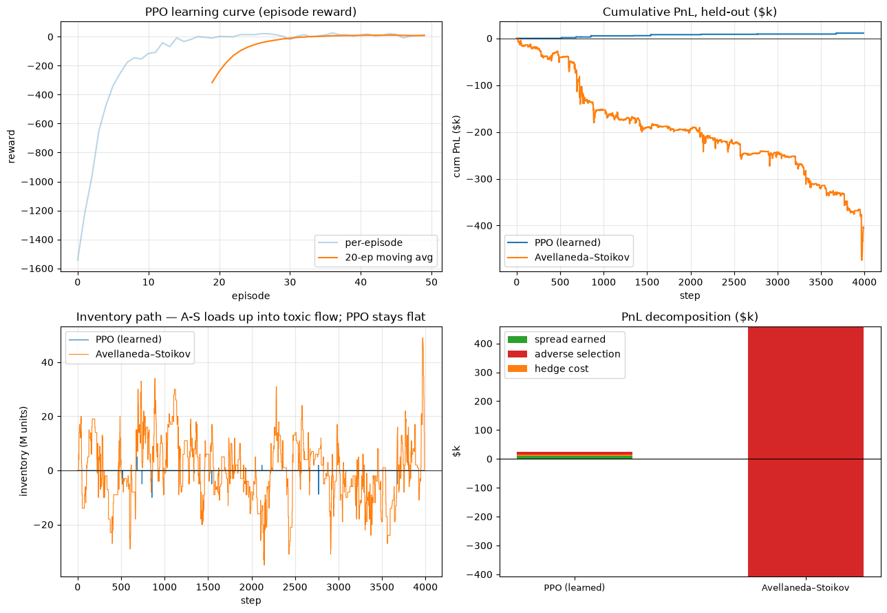
Takeaway: Avellaneda–Stoikov assumes uninformed flow, so it keeps quoting into the bursts and loads up to an inventory std of 11.6M — right as the mid drifts against it. Result: a net $-407,474 (adverse selection alone costs $-866,083). PPO sees the SAME market but also the burst intensity and signed-flow state in its observation, so it widens and hedges when flow turns toxic and keeps inventory std to 0.3M — netting $10,559. Look at the fill counts: A-S quotes into the toxicity 1004 times, PPO only 10 — it learned to *pull its quotes* when flow turns informed, exactly what a real desk does. PPO does not beat the market; it refuses to be the sucker on the other side of informed flow. That gap is the value of the state the closed form throws away. Real dealers add competition and per-client toxicity models on top — same idea, more state. Soften the toxicity and the optimal policy shifts from 'withdraw' to 'selectively quote in the calm, pull in the burst'.